Marginal Product of Labor
Marginal product of labor (MPL) is the increase in total production that occurs when labor increases by one unit, but all other inputs remain the same.
Firms care about marginal product of labor because their hiring decisions depend on whether the additional output generated by the new worker i.e. MPL is higher than the cost of the worker. If firms have enough demand for their goods, they continue hiring new workers as long as the revenue they generate i.e. their marginal product of labor is higher than their salary.
Calculation
Calculation of marginal product of labor depends on a firm or economy’s production function i.e. the relationship between labor, capital and output. For example, the Cobb-Douglas production function determines total output using the following formula:
$$ \text{Y}=\text{A}\times \text{K}^\alpha\times \text{L}^{\text{1}-\alpha} $$
Y is the total production i.e. the real value of an economy or firm’s production. A is the total factor productivity which shows the relationship between technology and production. K represents capital and L represents labor. α stands for the capital’s share in production i.e. the sensitivity of total production to capital.
Marginal product of labor is calculated using the following formula:
$$ \text{MPL}=(\alpha-\text{1})\times \text{A}\times \text{K}^\alpha\times \text{L}^{-\alpha}=\alpha\times\frac{\text{Y}}{\text{L}} $$
The formula above is derived by differentiating the Cobb-Douglas function with respect to labor while keeping capital constant.
$$ \text{MPL}=\frac{\partial \text{Y}}{\partial \text{L}}=\frac{\partial \text{A} \text{K}^\alpha \text{L}^{\text{1}-\alpha}}{\partial \text{L}} $$
$$ \text{MPL}=(\alpha-\text{1})\times \text{AK}^\alpha \text{L}^{\text{1}-\alpha-\text{1}} $$
Simplifying L1-α-1 and moving it to denominator:
$$ \text{MPL}=(\alpha-\text{1})\times \text{A}\times\frac{\text{K}^\alpha}{\text{L}^\alpha} $$
Multiplying and dividing the right-hand side of the above equation with L1-α, we get:
$$ \text{MPL}=(\alpha-\text{1})\times \text{A}\times\frac{\text{K}^\alpha}{\text{L}^\alpha}\times\frac{\text{L}^{\text{1}-\alpha}}{\text{L}^{\text{1}-\alpha}} $$
A bit of rearrangement:
$$ \text{MPL}=(\alpha-\text{1})\times\frac{\text{A}\times \text{K}^\alpha\times \text{L}^{\text{1}-\alpha}}{\text{L}^{\alpha+\text{1}-\alpha}} $$
From the definition of Cobb-Douglas production function, we conclude that the numerator equals Y. Similarly, the denominator simplifies to L:
$$ \text{MPL}=(\alpha-\text{1})\times\frac{\text{Y}}{\text{L}} $$
Graph and Example
Let’s consider an economy whose total production changes in response to changes in labor while keeping other inputs constant are shown in the table below.
| Number of Plants (K) | Number of Workers (L) | Total Production (Y) | Marginal Product of Labor |
|---|---|---|---|
| 1 | 0 | - | - |
| 1 | 100 | 200 | 200 |
| 1 | 200 | 283 | 83 |
| 1 | 300 | 346 | 64 |
| 1 | 400 | 400 | 54 |
| 1 | 500 | 447 | 47 |
| 1 | 600 | 490 | 43 |
| 1 | 700 | 529 | 39 |
| 1 | 800 | 566 | 37 |
This can be plotted as follows to observe the flattening marginal product of labor (MPL) curve.
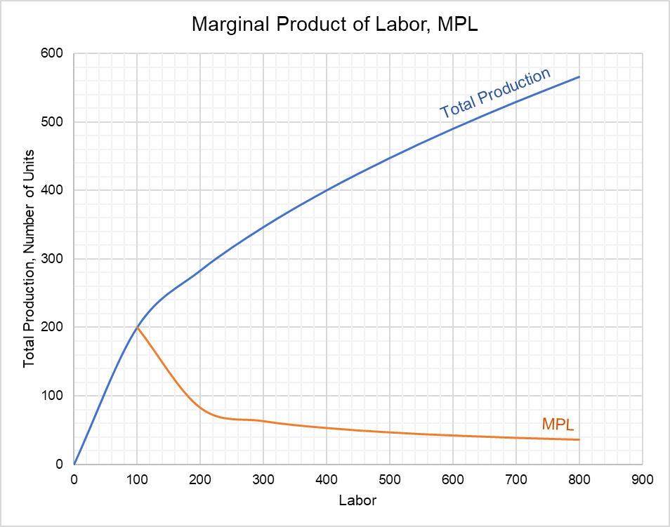
The marginal product of labor (MPL) decreases when capital is held constant. It is because under the constant returns of scale economy, a proportion between capital and labor must be maintained to achieve optimal production. When this condition is not met i.e. when one input (capital) is held constant and another (L) is allowed to increase, economy grows less impressively perhaps because there are too many workers but too few machines.
Firms also determine their marginal product of capital and compare it with their cost of capital to decide about their level of capital.
by Obaidullah Jan, ACA, CFA and last modified on