Economies of Scope
Economies of scope represent the production efficiency which enables a firm to produce more than one products at a cost which is lower than the sum of stand-alone costs of each product.
Economies of scope can occur, for example, when the by-product of a firm’s main production process can be used to produce another product cheaply, when the firm has a fixed resource such as a license which can be used to offer new products at minimal additional cost, when the firm’s supply chain can be leveraged to introduce another product at no additional cost, etc.
Example
Let’s consider a firm which operates a sugar mill. It processes 50,000 tons of sugar cane to produce 30,000 tons of sugar at a total cost of $15 million. The production process has a significant by-product which is sold at nominal price. If the firm decides to process the by-product in-house to produce ethyl alcohol, it would be able to produce 20,000 tons at a total cost of $3 million. Production of the same quantity of ethyl alcohol at a stand-alone facility would cost $6 million. This exhibits economies of scope because the firm can produce 30,000 tons of sugar and 20,000 tons of ethyl alcohol at a total cost of $18 million (=$15 million plus $3 million), which is lower than the combined stand-alone cost of sugar and ethyl alcohol i.e. $21 million (=$15 million plus $6 million).
Degree of economies of scope
Economies of scope exist when the combined cost of q1 and q2 is less than the sum of stand-alone cost of q1 and q2.
The degree of economies of scope is calculated using the following equation:
$$ \text{DSC}=\frac{\text{TC}(\text{q} _ \text{1})+\text{TC}(\text{q} _ \text{2})-\text{TC}(\text{q} _ \text{1} \text{,} \text{q} _ \text{2})}{\text{TC}(\text{q} _ \text{1} \text{,} \text{q} _ \text{2})} $$
If the degree of economies of scope is positive, scope economies exist, and it is better to produce the two products together. If the value is zero, there are neither economies of scope nor diseconomies of scope.
Graph
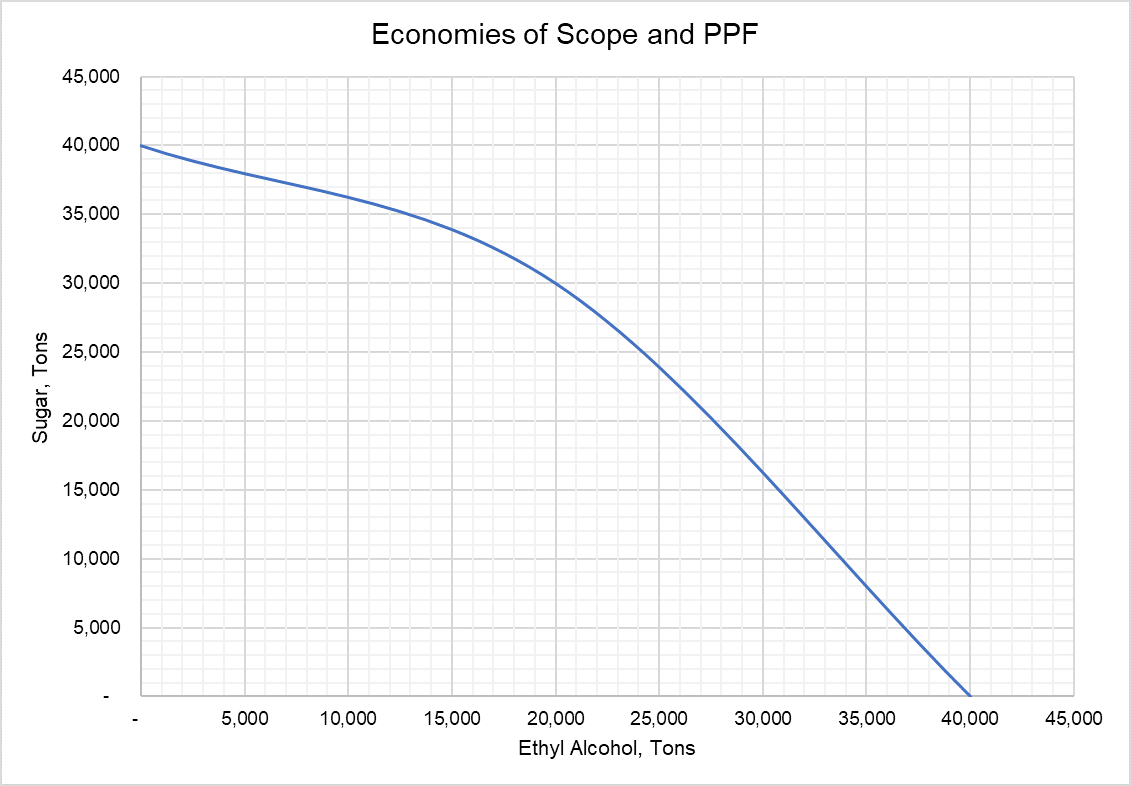
Economies of scope can be represented graphically by plotting a production possibility frontier. Where the economies of scope exist, the production possibility frontier is bowed out i.e. it is concave. This curve is also called product transformation curve.
Let’s modify our sugar mill example in terms of volume of inputs. Assume that the 50,000 tons of sugar cane can be processed by a sugar mill to produce 40,000 tons of sugar or by a chemical manufacturer to produce 40,000 tons of ethyl alcohol. But a single firm can use 50,000 tons to produce 30,000 tons of sugar and 20,000 tons of sugar. This shows that the combined output is higher as shown in the graph below.
Economies of scope vs diseconomies of scope
There might be a situation in which the combined production of two goods escalate the costs such that the combined cost of the two products is higher than the sum of the stand-alone costs of each product. Such a situation exhibits diseconomies of scope.
When the value of degree of economies of scope is negative, there are diseconomies of scope i.e. it is better to produce both products independently because the combined cost is higher than the sum of stand-alone costs.
by Obaidullah Jan, ACA, CFA and last modified on