Demand Function
A demand function is a mathematical equation which expresses the demand of a product or service as a function of the its price and other factors such as the prices of the substitutes and complementary goods, income, etc.
A demand functions creates a relationship between the demand (in quantities) of a product (which is a dependent variable) and factors that affect the demand such as the price of the product, the price of substitute and complementary goods, average income, etc., (which are the independent variables).
Let’s consider the market for ride-hailing apps and find out the factors that can affect the number of kilometers of ride-hailing services demanded by riders on a day. The most important factor is the price charged per kilometer. Other potential factors are the determinants of demand including price of substitutes i.e. price of the public transportation or competing cab services, whether it is a working day or a weekend, whether it is a clear or a rainy day, etc.
One method of creating a demand function to use multiple regression analysis to find out the relationship between quantity demanded, the product price and all other factors. The multiple regression analysis assigns different coefficients to each of the factor that affects the demand. The sign of the coefficient (i.e. positive or negative) tells us whether the demand and the factor are positively-related or negatively-related.
Let’s assume for the sake of simplification, you used only two variables : (a) price of the product itself and (b) the increase in price of the competing public transportation and arrived at the following equation:
$$ \text{Q}=\text{1,200,000}\ -\ \text{150,000}\times \text{P}+\text{200,000}\times \text{P} _ {\text{PT}} $$
Q is the kilometers demanded, P is the price per kilometer of ride-hailing service and PPT is the increase in price per ride of the public transit system. The P component has a negative sign which shows that with each dollar increase in charge per kilometer, quantity demanded will drop by 150,000 kilometers per day. The PPT component, on the other hand, has a positive sign, which means that a one dollar increase in public transport charge will result in increase in demand by 200,000 kilometers.
Since the equation above creates a relationship not only of the kilometers demanded with the price charged but also with the price of a substitute, it represents both a shift in the demand curve and a movement along the demand curve. As long as there is no change in the price of public transport, we can simplify the demand function to a relationship between Q and P:
$$ \text{Q}=\text{1,200,000}\ -\ \text{150,000}\times \text{P} $$
We can work out a demand schedule using the equation above just by plugging-in different prices per kilometer.
Inverse Demand Function
A supply and demand graph is typically plotted such that quantity is on x-axis and price is on y-axis but the demand function we defined above has price (P) as an independent variable and quantity (Q) as an independent variable.
Demand function is sometimes defined with price P as an independent variable. Such a demand function is called inverse demand function. With just a bith of mathematical manipulation, we can convert the demand function defined above to an inverse demand function:
$$ \text{150,000P}\ =\ \text{1,200,000}\ -\ \text{Q} $$
$$ \text{P}\ =\ \frac{\text{1,200,000}}{\text{150,000}}\ -\frac{\text{1}}{\text{150,000}}\ \text{Q} $$
$$ \text{P}\ =\ \text{8}\ -\frac{\text{1}}{\text{150,000}}\ \text{Q} $$
The inverse demand function is useful when we are interested in finding the marginal revenue, the additional revenue generated from one additional unit sold. Marginal revenue function is the first derivative of the inverse demand function. For inverse demand function of the form P = a – bQ, marginal revenue function is MR = a – 2bQ. Maginal revenue function in the above case is as follows:
$$ \text{MR}\ =\ \text{8}\ -\frac{\text{2}}{\text{150,000}}\ \text{Q} $$
Example
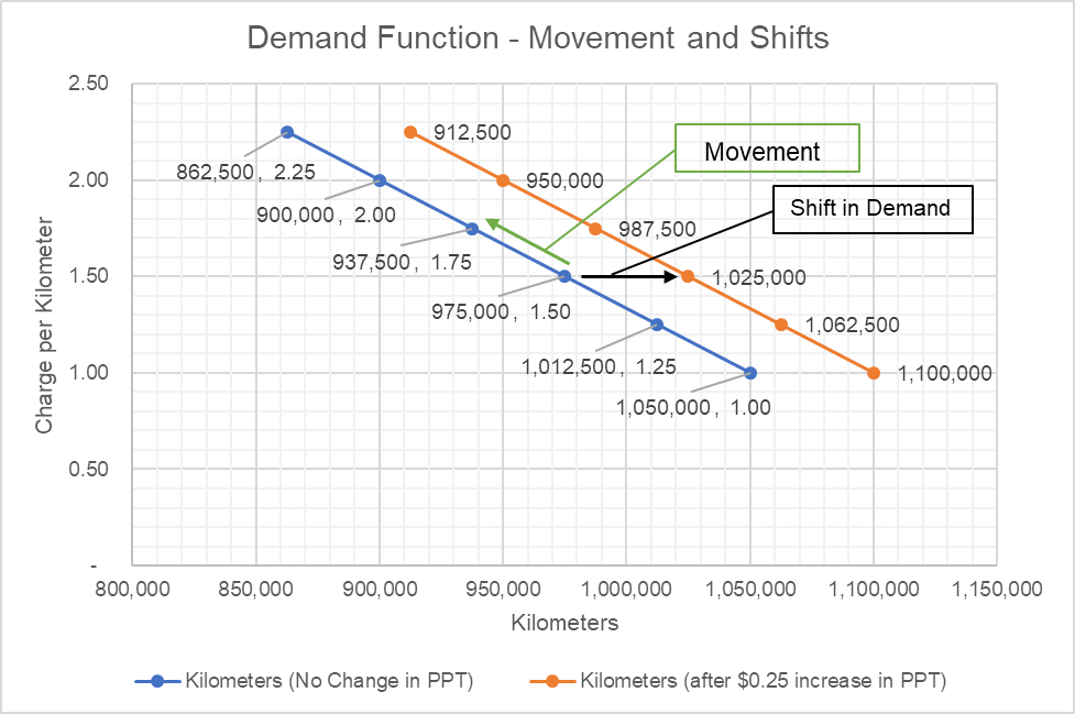
Let’s find out the kilometers demanded under the following scenarios: (a) the average price per kilometer (P) is $1.5 and $1.75; and (b) the average price per kilometer (P) is $1.5 and the increase in price of public transport (PPT) is $0.25
Scenario A
The following equation shows the quantity demanded corresponding to each price:
$$ \text{Q} _ {\text{1.50}}=\text{1,200,000}\ -\ \text{150,000}\times\text{\$1.50}=\text{975,000} $$
$$ \text{Q} _ {\text{1.75}}=\text{1,200,000}\ -\ \text{150,000}\times\text{\$1.75}=\text{937,500} $$
Scenario B
In this case, there is a change in price of substitute, so it represents a shift in the curve
$$ \text{Q} _ {\text{1.50};\text{0.25}}=\text{1,200,000}\ -\ \text{150,000}\times\text{\$1.50}+\text{200,000}\times\text{\$0.25}=\text{1,025,000} $$
As you can see the Q1.50;0.25 is higher than Q1.50 because the increase in public transit price has caused an outwards shift in the demand curve.
The following chart plots the movement along the initial demand curve in Scenario A and the shift in case of Scenario B
The demand function and the supply function can be used to solve for the market equilibrium and market clearing price.
by Obaidullah Jan, ACA, CFA and last modified on