Changes in Market Equilibrium
Market equilibrium occurs when the upward-sloping supply curve intersects the downward-sloping demand curve. When there is a change in supply and/or demand, quantity bought and sold in the market changes such that the market reached a new market clearing price.
Let’s consider the market for ride-hailing services where hundreds of drivers cater to thousands of consumers. Drivers supply more rides at higher fare per kilometer as shown by their upward-sloping supply curve.
$$ \text{Q} _ \text{s}=\text{2,500}\ +\text{7,500}\times \text{P}\ $$
Consumers, on the other hand, demand more rides at lower fares as evident from their downward-sloping demand curve.
$$ \text{Q} _ \text{d}=\text{50,000}\ -\ \text{10,000}\times \text{P} $$
When the rides supplied are higher than rides demanded, there is a surplus of drivers and the competition forces drivers to offer rides are lower prices which induces consumers to demand more rides and the market clears i.e. rides demanded equal rides supplied. Similarly, when there is a shortage, the scarcity lead drivers to bid their fares up which in turn reduces the rides demanded and clears the market. This market mechanism often referred to as the invisible hand is the engine that drives a market economy.
The equilibrium quantity and price can be worked out by solving the supply and demand functions or graphically by finding the point of intersection of demand and supply curves.
Movement vs Shift in Demand/Supply
If there is a change in price of a good, there is a change in quantity supplied and demanded but such a change represents a movement along the supply curve or demand curve. But when there is a change in any other determinant of supply or demand such as cost of production, price of substitute goods or complementary goods, etc., there is a shift in supply/demand curves i.e. there is a change in quantity at all prices.
In the example of ride-hailing services we discussed above, there can be a number of factors causing shifts in supply:
- increase in price of cars: inward (i.e. left-ward) shift in supply curve because due to high initial investment, fewer drivers sign up;
- increase in gas price: inward shift in supply due to increase in driving cost per km;
- increase in general unemployment: outward (i.e. rightward) shift in supply curve outwards because more people are be forced to consider this self-employment market;
Similarly, there are factors that will shift demand curve including:
- cost of comparable taxi services and public transportation: if price of substitutes is high, demand curve shifts outwards i.e. more is demanded at each price level;
- purchase price and lease cost of cars: outwards shift because it costly to own a car, hence more people consider using ride-hailing services;
- weather conditions: demand increases in bad weather because public transportation is inconvenient.
Example
Let’s assume it rains on a particular day, demand curve shifts such that the new demand curve is represented by the following equation:
$$ \text{Q} _ {\text{Nd}}=\text{60,000}\ -\ \text{9,000}\times \text{P} $$
Assuming that the supply curve remains the same, the following table shows old and new supply and demand schedule:
| Price ($) | Supply | Old Demand | New Demand |
|---|---|---|---|
| 0.50 | 6,250 | 45,000 | 55,500 |
| 1.00 | 10,000 | 40,000 | 51,000 |
| 1.50 | 13,750 | 35,000 | 46,500 |
| 2.00 | 17,500 | 30,000 | 42,000 |
| 2.50 | 21,250 | 25,000 | 37,500 |
| 3.00 | 25,000 | 20,000 | 33,000 |
| 3.50 | 28,750 | 15,000 | 28,500 |
| 4.00 | 32,500 | 10,000 | 24,000 |
These can be graphed as follows:
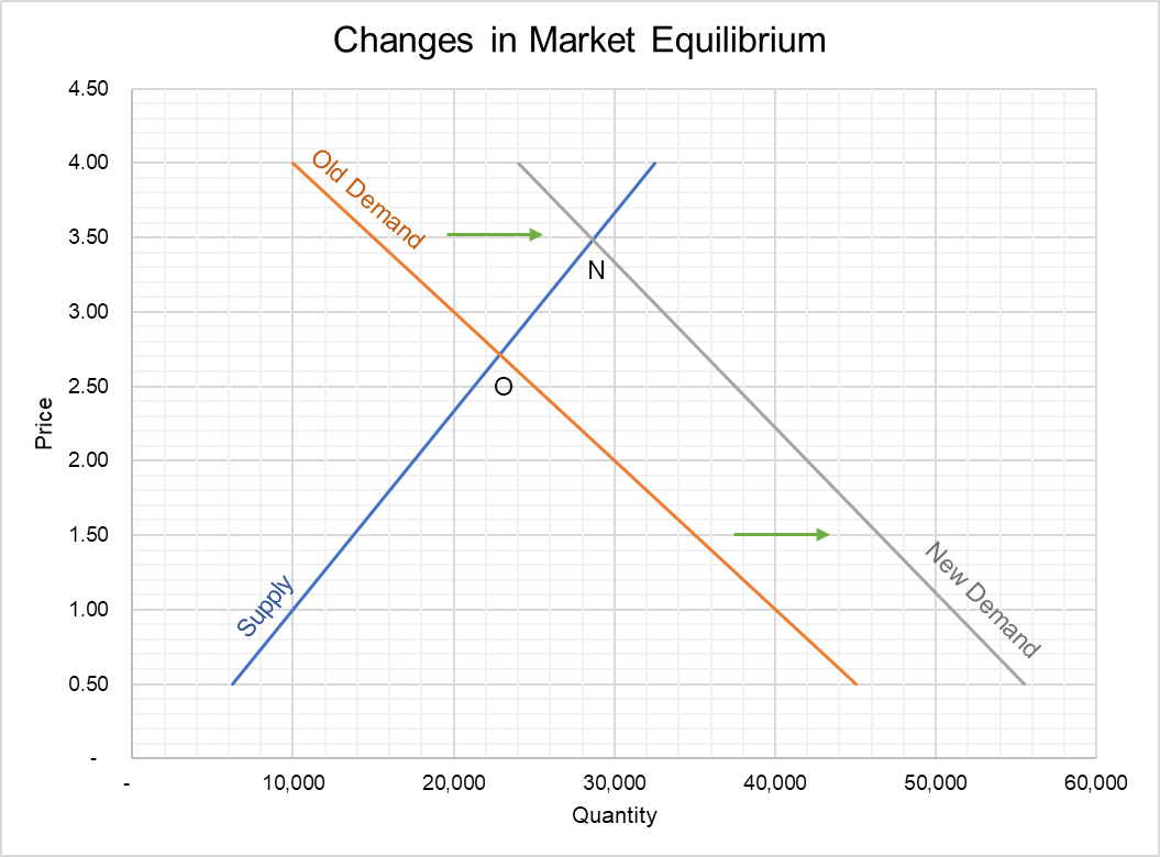
The initial market equilibrium is represented by Point O, the point of intersection of the Supply curve and Old Demand curve. It corresponds to a price of $2.71 and quantity (i.e. number of rides) of 22,857.
Due to right-ward shift in demand curve, the market equilibrium moves from Point O to Point N: the market clearing price increases to roughly $3.50 and the equilibrium quantity rises to a more than 28,000. We can use mathematics to calculate the exact market clearing price and quantity.
$$ \text{Q} _ \text{s}=\text{Q} _ {\text{Nd}} $$
$$ \text{2,500}\ +\text{7,500}\times \text{P}=\text{60,000}\ -\ \text{9,000}\times \text{P} $$
Moving all P terms to one side and constants to another:
$$ \text{7,500}\times \text{P}\ +\text{9,000}\times \text{P}=\text{60,000}\ -\ \text{2,500} $$
$$ \text{P}=\frac{\text{57,500}}{\text{16,500}}=\text{\$3.48} $$
Knowing the market clearing price, we can work out equilibrium quantity by substituting the value of P in either the supply function or demand function:
$$ \text{Q} _ {\text{Nd}}=\text{60,000}\ -\ \text{9,000}\times\text{\$3.48}=\text{28,636} $$
by Obaidullah Jan, ACA, CFA and last modified on