Income-Consumption Curve
Income-consumption curve is a graph of combinations of two goods that maximize a consumer’s satisfaction at different income levels. It is plotted by connecting the points at which budget line corresponding to each income level touches the relevant highest indifference curve.
The interplay of a consumer’s budget constraint and his indifference curves determine his utility-maximizing combination of goods. The point at which his budget constraint (which is derived from his income and prices of the relevant goods) is tangent to the highest indifference curve is the point at which a consumer’s utility is maximized.
One way in which this point of optimal consumption changes is when the consumer’s budget constraint shifts in response to change in income. If his income increases, his budget constraint shifts outwards (i.e. rightwards) enabling it to touch higher indifference curve thereby moving him to a new point of utility-maximization. Alternatively, if his income decreases and his budget line shifts inwards, he is forced to accept a consumption combination that lie on a lower indifference curve and so on. In order to keep track of the different optimal consumption pairs that correspond to difference income levels, we can draw a curve. This curve is called income-consumption curve. It is called income-consumption curve because it plots the movement of utility-maximizing consumption in response to changes in income.
Example
Let’s consider a Michael has to chose between hardcovers and paperbacks. His budget constraints and utility-optimizing consumption pairs are shown in the graph below. His initial budget constraint is represented by the blue line BL-1. He can spend his monthly income of $1,000 on 4 paperback but 0 hardcovers or 0 paperbacks and 2 hardcovers or any combination of both. If there is an increase in income, his budget constraint shifts outwards to BL-2 (showing income of $2,000) and then to BL-3 (corresponding to income of $3,000).
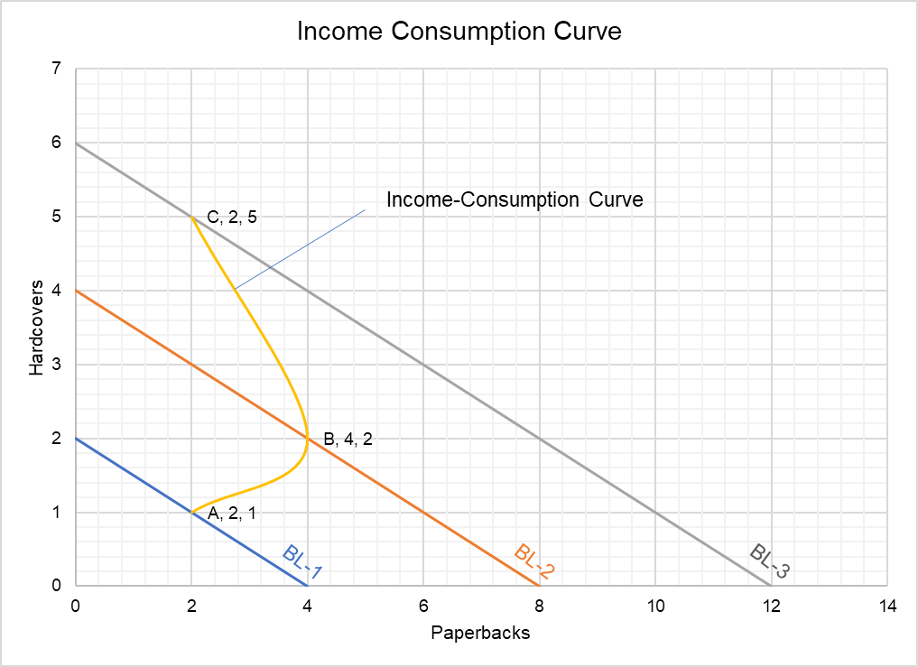
At income level of $1,000, his consumption preference is represented by Point A which corresponds to 2 paperbacks and 1 hardcover. It is the point of intersection of the highest indifference curve which the budget line BL-1 can touch. We have omitted the indifference curve from the diagram for the sake of simplicity. If his income increases to $2,000, his consumption choice moves to Point B. But as soon as income crosses the $2,000, his preference tilts towards hardcovers. At income level of $3,000 he reduces his consumption of paperbacks and increases consumption of hardcover. It shows that he considers hardcovers to be a normal good and paperbacks to be an inferior good.
The yellow line connecting Point A, Point B and Point C is the income-consumption curve. It can be used to create an Engel curve for Michael.
by Obaidullah Jan, ACA, CFA and last modified on