Second-Degree Price Discrimination
Second-degree price discrimination (also called nonlinear price discrimination) occurs when a firm charges different prices for different quantities of the product.
One of the conditions of (perfect) first-degree price discrimination is that the firm knows the reservation price of each unit that each of its customers consume. In most cases, firms do not have such detailed information about their customers, and they must infer reservation prices using some other measure. The law of diminishing marginal utility provides a useful insight: it tells us that the reservation price for the first unit must be higher than the second unit and so on because marginal utility decreases with increase in consumption. Second-degree price discrimination uses this insight in that it charges different prices for different number of units that a consumer buys.
Examples of second-degree price discrimination include quantity discounts, when more units are sold at a lower per-unit price; and block-pricing, when the consumer pays different price for different blocks of a product say electricity, gas, internet, etc.
Example
Let’s consider Varys Communications, a telecommunication company. The company’s inverse demand function (showing price per GB of data) is as follows:
$$ \text{P}\ =\ \text{\$5}\ -\ \text{0.25Q} $$
Since the slope of the marginal revenue curve is double that of the demand curve, the marginal revenue function can be written as follows:
$$ \text{MR}\ =\ \text{\$5}\ -\ \text{0.5Q} $$
If the marginal cost of a GB of data is constant $2, optimal output occurs when P = $3.5 and quantity is 6 GB.
The following graph shows what happens when there is no price discrimination.
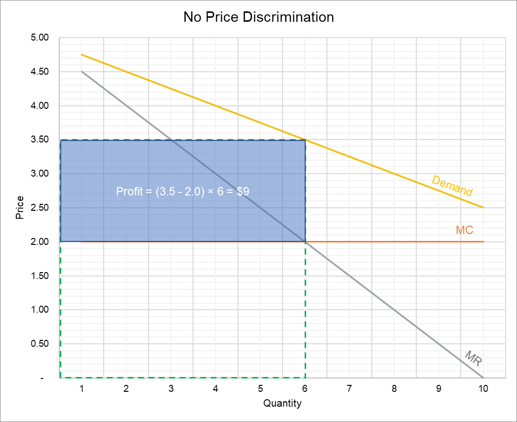
The green-dashed rectangle shows total revenue (which is $21 on average) and the blue-shaded rectangle shows profit of $9 (=$21-6×$2).
When a firm engages in price discrimination, the marginal revenue curve is no longer relevant. It is because the firm doesn’t need to reduce its price in order to sell more output. It means that a firm engaging in price discrimination should produce as long as the price is higher than the marginal cost.
Additional Profit
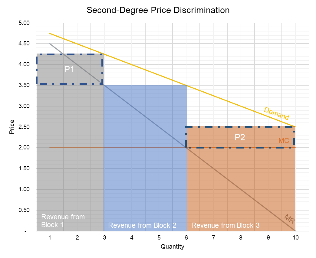
Let’s see what happens if Varys charges $4.25/GB for 1-3 GB, $3.5/GB for 4-6 GB and $2.5/GB for 7-10 GBs.
Under the new block-pricing, total revenue is $33.25 (=3 × $4.25 + 3 × $3.5 + 4 × $2.5). Since the marginal cost for 10 GB is $20 (=$2×10), profit is $13.25 (=$33.25 - $20).
The following graph shows how second-degree price discrimination works:
Change in Consumer and Producer Surplus
The grey, blue and red shaded areas show revenues from the first, second and third blocks of the data plan. Additional profit equals the sum of the areas of rectangles P1 and P2. You can verify that it equals $4.25 (=$13.25 - $9).
Rectangle P1 represents the consumer surplus which has been captured by the producer. P3 shows the net increase in welfare due to price discrimination. The white unshaded triangles under the demand curve show consumer surplus which still remains. In perfect first-degree price discrimination, all the consumer surplus is converted to producer surplus.
by Obaidullah Jan, ACA, CFA and last modified on