Equity Beta
Equity beta (or just beta) is a measure of a stock’s systematic risk. It is estimated by comparing the sensitivity of a stock’s return to the broad market return. Under the capital asset pricing model, cost of equity equals risk free rate plus the market risk premium multiplied by the stock’s beta. The broad market has a beta of 1 and a stock’s beta of less than 1 means that it has lower systematic risk than the market and vice versa.
There are three types of beta coefficients: equity beta (also called levered or geared beta), debt beta and asset beta (also called unlevered or ungeared beta). Equity beta is the most common and is referred to as just beta in most cases. Major finance websites such as Yahoo Finance, Google Finance, Bloomberg, etc. quote equity beta values.
Beta coefficient (specifically the equity beta) is a measure of how severely an investment is exposed to the systematic risk. Systematic risk is the risk of major economy-wide effects such as interest rate hike, war, etc. that affect the whole system and not just individual stocks. In a portfolio context, systematic risk is important because it can't be diversified and must be priced.
The market beta i.e. the average beta of all the investments that are out there is 1 and an individual investment’s systematic risk is measured relative to the overall market risk. A beta of more than 1 means that the investment has higher exposure to systematic risk than the market in general and a beta less than 1 means that the investment is less exposed to the systematic risk factors.
Calculating Beta
In the capital asset pricing model, required return on a stock (or portfolio of stocks) is determined using the following equation:
$$ \text{r}=\text{r} _ \text{f}+\beta\times(\text{r} _ \text{m}-\text{r} _ \text{f}) $$
Where r is the required return on equity (i.e. cost of equity), rf is the risk-free rate, rm is the return on the broad market index and β is the beta.
The above equation can be graphed, and the graph is called the security market line which plots the expected return on y-axis against beta values on x-axis. Beta is the slope of that line.
You can determine beta by either (a) regressing the investment return on the broad market index or (b) finding slope of the security market line or (c) calculating it directly using the following formula given the covariance of the investment returns and market returns and variance of the market returns.
$$ \beta=\frac{\text{Covariance}(\text{r} _ \text{i} \text{,} \text{r} _ \text{m})}{{\sigma _ \text{m}}^\text{2}} $$
Where σm2 is the variance of the market returns.
We know that covariance(ri, rm) equals the product of standard deviation of investment returns (σi), standard deviation of market (σm) and correlation coefficient (ρ). Substituting covariance (ri, rm) in the above equation, we get the following formula:
$$ \beta=\frac{\sigma _ \text{i}\sigma _ \text{m}\rho}{{\sigma _ \text{m}}^\text{2}}=\frac{\sigma _ \text{i}}{\sigma _ \text{m}}\rho $$
Example: Calculating Beta with Regression, SLOPE Function and Formula
Let’s determine beta of Tesla (NASDAQ: TSLA). We need a history of the company’s stock prices and corresponding values of some broad market index, say S&P 500. We can obtain these values from major financial news websites such as Yahoo Finance. Beta is dependent on the time period and reporting frequency (daily, weekly or monthly). Further, the time duration and frequency of stock prices and index values must match. The following table shows relevant stock values, index values and associated returns calculated using the holding period return formula.
| Date | TSLA Price | TSLA Return | S&P 500 Index | S&P 500 Return |
|---|---|---|---|---|
| 4/3/2017 | 302.54 | 2,355.54 | ||
| 4/10/2017 | 304.00 | 0.48% | 2,328.95 | -1.13% |
| 4/17/2017 | 305.60 | 0.53% | 2,348.69 | 0.85% |
| 4/24/2017 | 314.07 | 2.77% | 2,384.20 | 1.51% |
| 5/1/2017 | 308.35 | -1.82% | 2,399.29 | 0.63% |
| 5/8/2017 | 324.81 | 5.34% | 2,390.90 | -0.35% |
| 5/15/2017 | 310.83 | -4.30% | 2,381.73 | -0.38% |
| 5/22/2017 | 325.14 | 4.60% | 2,415.82 | 1.43% |
| 5/29/2017 | 339.85 | 4.52% | 2,439.07 | 0.96% |
| 6/5/2017 | 357.32 | 5.14% | 2,431.77 | -0.30% |
| 6/12/2017 | 371.40 | 3.94% | 2,433.15 | 0.06% |
| 6/19/2017 | 383.45 | 3.24% | 2,438.30 | 0.21% |
| 6/26/2017 | 361.61 | -5.70% | 2,423.41 | -0.61% |
| 7/3/2017 | 313.22 | -13.38% | 2,425.18 | 0.07% |
| 7/10/2017 | 327.78 | 4.65% | 2,459.27 | 1.41% |
| 7/17/2017 | 328.40 | 0.19% | 2,472.54 | 0.54% |
| 7/24/2017 | 335.07 | 2.03% | 2,472.10 | -0.02% |
| 7/31/2017 | 356.91 | 6.52% | 2,476.83 | 0.19% |
| 8/7/2017 | 357.87 | 0.27% | 2,441.32 | -1.43% |
| 8/14/2017 | 347.46 | -2.91% | 2,425.55 | -0.65% |
| 8/21/2017 | 348.05 | 0.17% | 2,443.05 | 0.72% |
| 8/28/2017 | 355.40 | 2.11% | 2,476.55 | 1.37% |
| 9/4/2017 | 343.40 | -3.38% | 2,461.43 | -0.61% |
| 9/11/2017 | 379.81 | 10.60% | 2,500.23 | 1.58% |
| 9/18/2017 | 351.09 | -7.56% | 2,502.22 | 0.08% |
| 9/25/2017 | 341.10 | -2.85% | 2,519.36 | 0.68% |
| 10/2/2017 | 356.88 | 4.63% | 2,549.33 | 1.19% |
| 10/9/2017 | 355.57 | -0.37% | 2,553.17 | 0.15% |
| 10/16/2017 | 345.10 | -2.94% | 2,575.21 | 0.86% |
| 10/23/2017 | 320.87 | -7.02% | 2,581.07 | 0.23% |
| 10/30/2017 | 306.09 | -4.61% | 2,587.84 | 0.26% |
| 11/6/2017 | 302.99 | -1.01% | 2,582.30 | -0.21% |
| 11/13/2017 | 315.05 | 3.98% | 2,578.85 | -0.13% |
| 11/20/2017 | 315.55 | 0.16% | 2,602.42 | 0.91% |
| 11/27/2017 | 306.53 | -2.86% | 2,642.22 | 1.53% |
| 12/4/2017 | 315.13 | 2.81% | 2,651.50 | 0.35% |
| 12/11/2017 | 343.45 | 8.99% | 2,675.81 | 0.92% |
| 12/18/2017 | 325.20 | -5.31% | 2,683.34 | 0.28% |
| 12/25/2017 | 311.35 | -4.26% | 2,673.61 | -0.36% |
| 1/1/2018 | 316.58 | 1.68% | 2,743.15 | 2.60% |
| 1/8/2018 | 336.22 | 6.20% | 2,786.24 | 1.57% |
| 1/15/2018 | 350.02 | 4.10% | 2,810.30 | 0.86% |
| 1/22/2018 | 342.85 | -2.05% | 2,872.87 | 2.23% |
| 1/29/2018 | 343.75 | 0.26% | 2,762.13 | -3.85% |
| 2/5/2018 | 310.42 | -9.70% | 2,619.55 | -5.16% |
| 2/12/2018 | 335.49 | 8.08% | 2,732.22 | 4.30% |
| 2/19/2018 | 352.05 | 4.94% | 2,747.30 | 0.55% |
| 2/26/2018 | 335.12 | -4.81% | 2,691.25 | -2.04% |
| 3/5/2018 | 327.17 | -2.37% | 2,786.57 | 3.54% |
| 3/12/2018 | 321.35 | -1.78% | 2,752.01 | -1.24% |
| 3/19/2018 | 301.54 | -6.16% | 2,588.26 | -5.95% |
| 3/26/2018 | 266.13 | -11.74% | 2,640.87 | 2.03% |
Once we have all the data ready, we can use any of the following methods: (a) slope function, (b) regression analysis and (c) manual calculation. Use Excel SLOPE function, selecting the range of Tesla return values as the knownys argument and S&P 500 return values as the knownxs argument. You will get a value of 1.068.
For the regression analysis, (a) you need to enable Excel Analysis Toolpack in Options, (b) select “data analysis” from data tab, (c) select “Regression” in the dialogue box, (d) enter Tesla return values as Y and S&P 500 return values as X and (e) get the following ouput:
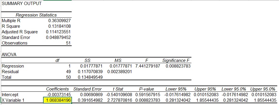
Instead of the raw data, if you just had values for standard deviation of Tesla stock of 5.19%, S&P 500 of 1.76% and correlation coefficient between Tesla and S&P500 of 0.363, you could have worked out Tesla’s beta using the formula approach as follows:
$$ \beta=\frac{\sigma _ \text{i}}{\sigma _ \text{m}}\rho=\frac{\text{5.19%}}{\text{1.76%}}\times\text{0.363}=\text{1.07} $$
So what does a beta coefficient of 1.07 means? It means that Tesla has a slightly higher exposure to systematic risk than the S&P500 index as a whole. If the risk free rate is 4% and the market return is 9%, Tesla's cost of equity can be determined using the capital asset pricing model as follows:
$$ \text{Tesla k} _ \text{e}=\text{r} _ \text{f}+\beta\times(\text{r} _ \text{m}-\text{r} _ \text{f})=\text{4%}+\text{1.068}\times(\text{9%}-\text{4%})=\text{9.7%} $$
Negative Beta
A negative beta means that the investment or investment portfolio behaves inversely to the broad market. It means that when the broad market performs poorly due to systematic factors, the investment with negative beta generates positive returns and vice versa. One plausible example is that of gold or stocks of companies engaged in exploration or trading of gold. When the stock market in general is performing poorly, people seek safety in gold and it is expected that the gold should generate positive returns when the stock market is yielding negative returns.
Adjusted beta
The beta estimated using the historical data is not necessarily the best indicator of future systematic risk and expected return. Due to the tendency of beta to revert to the mean value of 1, adjusted beta is normally used for future periods.
Adjusted beta is calculated using the following formula:
$$ \text{Adjusted Beta}\ (\beta _ {\text{adj}})=\text{0.66}\times\beta _ \text{h}+\text{0.33}\times\text{1} $$
Where βadj is the adjusted beta and βh is the historical equity beta.
Looking at the Tesla’s example above, it’s adjusted beta would be 1.035:
$$ \text{Adjusted Beta}\ (\beta _ {\text{adj}})=\text{0.66}\times\text{1.068}+\text{0.33}\times\text{1}=\text{1.035} $$
The adjustment in this example is not very pronounced because the historical beta is already close to 1. The adjustment is most visible in case of beta values which stray away from 1.
by Obaidullah Jan, ACA, CFA and last modified on