Capital Market Line
Capital market line is the graph of the required return and risk (as measured by standard deviation) of a portfolio of a risk-free asset and a basket of risky assets that offers the best risk-return trade-off. It is a special case of capital allocation line that is tangent to the efficient frontier and the slope of the capital allocation line represents the Sharpe ratio.
You might want to review the article on risk and return to obtain an understanding of the portfolio expected return, portfolio standard deviation and their interplay using the efficient frontier.
A well-diversified portfolio of risky assets has zero unsystematic risk. The point on efficient frontier that has the lowest risk is called the global minimum variance portfolio. If an investor has an option to borrow and lend at the risk-free rate, he can create an asset allocation which is a mix of the risk-free asset and the portfolio of risky portfolio.
Risk-free asset is an asset that has zero risk i.e. zero standard deviation. US treasury securities can be considered risk-free assets for this analysis.
Expected return of a portfolio of a risk-free asset and a portfolio of risky asset can be determined using the following formula:
$$ \text{E}(\text{R})=\text{w} _ \text{r}\times \text{r} _ \text{f}+(\text{1}-\text{w} _ \text{r})\times \text{r} _ \text{p} $$
Where wr is the weight of the risk-free asset, rf is the risk-free rate of return and rp is the return on the portfolio of risky assets.
Standard deviation of a portfolio of risk-free asset and risky assets can be expressed using the following equation:
$$ \sigma=\sqrt{\text{w}^\text{2}{\sigma _ \text{r}}^\text{2}+{(\text{1}-\text{w})}^\text{2}{\sigma _ \text{p}}^\text{2}+\text{2w}(\text{1}-\text{w})\sigma _ \text{r}\sigma _ \text{p}\rho} $$
Where w is weight of the risk-free asset, σr is standard deviation of risk-free asset, σp is the standard deviation of the portfolio of risky assets and ρ is the correlation coefficient of returns of risk-free asset and the portfolio of risky assets.
Because a risk-free asset has zero standard deviation and its correlation with a portfolio of risky asset is zero, the above equation can be simplified as follows:
$$ \sigma=\sqrt{{(\text{1}-\text{w})}^\text{2}{\sigma _ \text{p}}^\text{2}} $$
After some mathematical manipulation we can arrive at the following equation which represents the capital allocation line:
$$ \text{E}(\text{R})=\text{r} _ \text{f}+\frac{\text{E}(\text{R})-\text{r} _ \text{f}}{\sigma _ \text{P}}\times\sigma $$
Where E(R) is the expected return on the portfolio of the risk-free asset and risky assets, rf is the risk-free rate, σP is the standard deviation of the portfolio of risky assets and σ is the standard deviation of the new portfolio (comprising of both the risk-free rate and the risky assets). The factor of (E(R) – rf)/σP) measures the return in addition to the risk-free rate per unit of risk. It is also called rewards-to-risk ratio. It is the slope of the capital allocation line.
Example
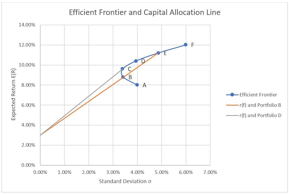
In the example of efficient frontier, we identified a set of portfolios that offer same risk-return trade-off. Let’s combine risk-free asset with expected return of 3% with the portfolio B and D.
The following table shows the expected return and standard deviation of Portfolio B and D:
| Portfolio | Portfolio Standard Deviation | Portfolio Expected Return |
|---|---|---|
| B | 4.87% | 11.20% |
| D | 3.39% | 9.60% |
The following shows the expected return and standard deviation of a mix of risk-free asset and portfolios B and D:
| Weight of Risk-Free Asset | E(R) of Rf and Portfolio B | σ of rf and Portfolio B | E(R) of Rf and Portfolio D | σ of rf and Portfolio D |
|---|---|---|---|---|
| 100% | 3.00% | 0.00% | 3.00% | 0.00% |
| 80% | 4.64% | 0.97% | 4.32% | 0.68% |
| 60% | 6.28% | 1.95% | 5.64% | 1.36% |
| 40% | 7.92% | 2.92% | 6.96% | 2.03% |
| 20% | 9.56% | 3.89% | 8.28% | 2.71% |
| 0% | 11.20% | 4.87% | 9.60% | 3.39% |
Let’s plot these values on top of the efficient frontier graph:
Capital Allocation Line vs Capital Market Line
The captial allocation line is a graph that represents the risk and return profile of a portfolio that is a combination of the risk-free rate and ANY portfolion on the efficient frontier. Both the lines in the above graphs (representing the combination of risk-free asset and Portfolio C and risk-free asset and Portfolio D) are capital allocation lines.
The capital allocation line representing the mix of risk-free asset and Portfolio D (let’s call it CAL 1) is superior to the capital allocation line of risk-free asset and Portfolio B (let’s call it CAL 2). It is called the capital market line and it is the best possible way in which the risk-free rate and a portfolio of risky assets can be mixed. This is because at all risk levels i.e. standard deviation levels, CAL 1 offers a higher return. The portfolio at the intersection of the efficient frontier and the capital allocation line is the optimal portfolio.
Capital market line is a pre-cursor to the security market line.
by Obaidullah Jan, ACA, CFA and last modified on