Cournot Model
Cournot model is an oligopoly model in which firms producing identical products compete by setting their output under the assumption that its competitors do not change their output in response.
Unlike a monopoly in which there is only one producer, an oligopoly in a market structure in which there are more than one producer, and each is large enough to affect the profit of other firms through its actions. Let’s assume that Reach and Dorne are the only two producers of cotton in Westeros. If the total demand is 20 thousand tons per annum and Reach produces 15 thousand tons in one period, there is only 5 thousand tons left for Dorne to produce. If Dorne produces more than 5 thousand tons, the market price will drop hurting both Reach and Dorne. Cournot model helps us determine such an output level for an oligopoly at which no firm is better off by changing its output unilaterally.
If Q is the total output, which is sum of QR, the quantity produced by Reach and QD, the quantity produced by Dorne, the demand function for cotton can be written as follows:
$$ \text{P}\ =\ \text{2,000}\ -\ \text{20}\times \text{Q} $$
$$ \text{P}=\text{2,000}-\text{20}\times\left(\text{Q} _ \text{R}+\text{Q} _ \text{D}\right) $$
$$ \text{P}=\text{2,000}-\text{20Q} _ \text{R}-\text{20Q} _ \text{D} $$
The profit-maximizing output of the oligopoly as a whole occurs when marginal revenue is equal to marginal cost.
Let’s assume that marginal cost is $1,500 in Reach and $1,600 in Dorne.
Marginal revenue function for Reach can be determined by finding the total revenue function (as a product of Q and P) and then obtaining its first derivative with respect to QR:
$$ {\text{MR}} _ \text{R}=\text{2,000}-\text{40Q} _ \text{R}\ -\ \text{20Q} _ \text{D} $$
Similarly, the marginal revenue function for Dorne is as follows:
$$ {\text{MR}} _ \text{D}=\text{2,000}-\text{20Q} _ \text{R}\ -\ \text{40Q} _ \text{D} $$
Residual Demand Curve
Going back to our example we see that if Reach produces 15 tons, the demand function for Dorne can be written as follows:
$$ \text{P}=\text{2,000}-\text{20}\times\text{15}\ -\ \text{20Q} _ \text{D}=\text{1,700}\ -\ \text{20Q} _ \text{D} $$
The equation above is a function of a residual demand curve. A residual demand curve is a demand curve which shows the demand left over for a firm given the supply of other firms.
If Reach produces 20 tons, Dorne’s residual demand curve reduces to P = 1,600 – 20QD and so on.
Using the residual demand curve, we can find out the residual marginal revenue curve. One short-cut is to double the slope of the line (because MR curve has twice the slope of the demand curve).
$$ \text{MR}=\text{1,700}\ -\ \text{40Q} _ \text{D} $$
Using the MR = MC condition, we get the profit-maximizing output for Dorne given Reach’s output of 15 tons as follows:
$$ \text{1,600}=\text{1,700}\ -\ \text{40Q} _ \text{D} $$
$$ \text{Q} _ \text{D}=\text{2.5}\ $$
Similarly, if Reach’s output is 20 tons, Dorne’s optimal output is 0
$$ \text{1,600}=\text{1,600}\ -\ \text{40Q} _ \text{D} $$
$$ \text{Q} _ \text{D}=\text{0} $$
It shows that Dorne’s profit-maximizing output changes when output of its rival changes. But Reach is also facing the same dilemma and its profit-maximizing output changes when Dorne’s output changes.
Reaction Curve or Best-Response Curve
A reaction curve (or best-response curve) is a graph which shows profit-maximizing output of one firm in a duopoly given the output of the other firm. We can obtain a firm’s reaction curve using the MRR = MCR condition.
$$ \text{1,500}=\text{2,000}-\text{40Q} _ \text{R}\ -\ \text{20Q} _ \text{D} $$
$$ \text{Q} _ \text{R}=\text{12.5}\ -\ \text{0.5Q} _ \text{D} $$
The equation above expresses the output of Reach in terms of output of Dorne. It shows that both QR and QD are inversely-related. If Dorne increases output, Reach must decrease its own.
Using the same steps i.e. MRD = MCD, we can find that the profit-maximizing output for Dorne:
$$ \text{1,600}=\text{2,000}-\text{20Q} _ \text{R}\ -\ \text{40Q} _ \text{D} $$
$$ \text{Q} _ \text{D}=\text{10}\ -\ \text{0.5Q} _ \text{R} $$
If we plug different values of QR, we get the following QD values:
| QR | QD |
|---|---|
| 0 | 10 |
| 5 | 7.5 |
| 10 | 5 |
| 15 | 2.5 |
| 20 | 0 |
This table shows output of Dorne given output of Reach. If we plot this data, we get Dorne’s reaction curve.
We can create a similar table for Reach (given Dorne’s output). If we plot both these data series, we get the following graph:
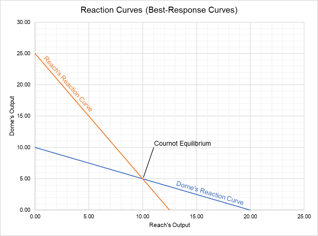
Cournot Equilibrium
Cournot equilibrium is the output level at which all firms in an oligopoly have no incentive to change their output. It is the point of intersection of the best-response curves of the rivals in a duopoly.
Since both firms need to take the output decision simultaneously, we can find the equilibrium by solving reaction curves of both firms.
Substituting the value of QR from Reach’s reaction curve in Dorne’s reaction curve, we get:
$$ \text{Q} _ \text{D}=\text{10}\ -\ \text{0.5}\times(\text{12.5}\ -\ \text{0.5Q} _ \text{D}) $$
$$ \text{Q} _ \text{D}=\text{10}\ -\ \text{6.25}\ +\ \text{0.25Q} _ \text{D} $$
$$ \text{Q} _ \text{D}=\text{5} $$
Substituting QD in the reaction curve for Dorne, we find that QR is 10.
$$ \text{Q} _ \text{R}=\text{12.5}\ -\ \text{0.5}\times\text{5}=\text{10} $$
The oligopoly price that corresponds to Cournot equilibrium is 1,666.8.
$$ \text{P}=\text{2,000}-\text{20}\times\left(\text{5}+\text{10}\right)=\text{1,700} $$
Comparison: Cournot vs Bertrand vs Collusion
Cournot equilibrium tells us that an oligopoly which produces identical products, and which compete based on output will produce a higher output than a monopoly but lower output than a Bertrand oligopoly. It will charge a lower price than a monopoly but a higher price than a Bertrand oligopoly.
Cournot model also tells us that a firm in an oligopoly with lower marginal cost will produce a higher output and will have a higher market share. This is evident from the example above: Reach has lower marginal cost and higher share of the output in Cournot equilibrium.
by Obaidullah Jan, ACA, CFA and last modified on