Cost Curves
Cost curves are graphs of how a firm’s costs change with change in output. Economists draw separate curves for short-run and long-run because firms have higher flexibility in selecting their inputs in the long-run.
Differentiating between short-run and long-run cost curves is important because in the short-run at least one of the inputs is fixed. When an input, say capital, is fixed, the marginal product of all other inputs, say labor, ultimately exhibit the law of diminishing returns in the short-run. Since a firm is able to vary all inputs in the long-run, the long-run cost curves depends on the firm’s returns to scale, economies of scale and economies of scope.
Short-run Cost Curves
A firm’s total costs can be broadly categorized as either fixed or variable. Fixed costs are costs which a firm incur regardless of the output level. These costs do not change with change in output. Variable costs, on the other hand, are costs which vary directly with output. The relationship between a firm’s total costs (TC), fixed costs (FC) and variable costs (VC) can be written as follows:
$$ \text{TC}\ =\ \text{FC}\ +\ \text{VC} $$
If we divide both sides of the above equation with Q, we get the relationship between average costs:
$$ \frac{\text{TC}}{\text{Q}}\ =\ \frac{\text{FC}}{\text{Q}}\ +\ \frac{\text{VC}}{\text{Q}} $$
It shows that the average total cost (TC/Q) is the sum of average fixed cost (FC/Q) and average variable cost (VC/Q).
Marginal cost is the incremental cost of each additional unit. It equals total cost at Q units minus total cost at Q – 1 units. Alternatively, it can also be defined as total variable cost at Q units minus total variable cost at Q – 1 units. Marginal cost equals the slope of the total cost curve and it can be calculated using the following formula:
$$ \text{MC}=\frac{\Delta \text{TC}}{\Delta \text{Q}} $$
Example
Let’s consider a firm whose cost structure is represented by the following table:
| Quantity | TC | FC | VC | MC | ATC | AFC | AVC |
|---|---|---|---|---|---|---|---|
| 0 | 15 | 15 | - | ||||
| 1 | 25 | 15 | 10 | 10.00 | 25.00 | 15.00 | 10.00 |
| 2 | 34 | 15 | 19 | 9.00 | 17.00 | 7.50 | 9.50 |
| 3 | 42 | 15 | 27 | 8.10 | 14.03 | 5.00 | 9.03 |
| 4 | 49 | 15 | 34 | 7.29 | 12.35 | 3.75 | 8.60 |
| 5 | 56 | 15 | 41 | 6.56 | 11.19 | 3.00 | 8.19 |
| 6 | 62 | 15 | 47 | 5.90 | 10.31 | 2.50 | 7.81 |
| 7 | 67 | 15 | 52 | 5.31 | 9.60 | 2.14 | 7.45 |
| 8 | 73 | 15 | 58 | 5.85 | 9.13 | 1.88 | 7.25 |
| 9 | 79 | 15 | 64 | 6.43 | 8.83 | 1.67 | 7.16 |
| 10 | 87 | 15 | 72 | 7.07 | 8.65 | 1.50 | 7.15 |
| 11 | 94 | 15 | 79 | 7.78 | 8.57 | 1.36 | 7.21 |
| 12 | 103 | 15 | 88 | 8.56 | 8.57 | 1.25 | 7.32 |
| 13 | 112 | 15 | 97 | 9.41 | 8.64 | 1.15 | 7.48 |
| 14 | 123 | 15 | 108 | 10.36 | 8.76 | 1.07 | 7.69 |
| 15 | 134 | 15 | 119 | 11.39 | 8.93 | 1.00 | 7.93 |
| 16 | 147 | 15 | 132 | 12.53 | 9.16 | 0.94 | 8.22 |
| 17 | 160 | 15 | 145 | 13.78 | 9.43 | 0.88 | 8.55 |
| 18 | 176 | 15 | 161 | 15.16 | 9.75 | 0.83 | 8.92 |
| 19 | 192 | 15 | 177 | 16.68 | 10.11 | 0.79 | 9.33 |
| 20 | 211 | 15 | 196 | 18.35 | 10.53 | 0.75 | 9.78 |
If we plot average total cost, average fixed cost, average variable cost and marginal cost, we get the following chart:
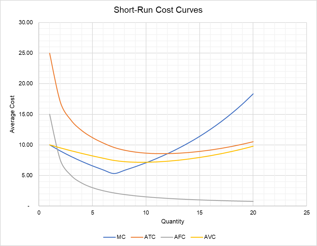
We can draw some general conclusions from the cost curves plotted above:
- The average fixed cost (AFC) decreases continuously with increase in output. Since AFC = TC/Q, increase in Q decreases AFC indefinitely.
- The average variable cost (AVC) curve is U-shaped. It slopes downward as long as the marginal cost curve is below AVC, but it starts to slope upwards when the marginal cost curve crosses it from below. It is because the AVC is effectively the average of the cumulative marginal cost.
- The marginal cost curve is U-shaped. It initially decreases when marginal product increases, but it starts to rise as the diminishing returns set in.
- AVC is equal to MC at the output level at which AVC intersects MC.
- The average total cost (ATC) curve is the vertical sum of the average fixed cost (AFC) curve and average variable cost (AVC) curve.
Long-run Cost Curves
Since all inputs, both labor and capital, are variable in the long-run, the long-run cost structure depends on the firm’s expansion path, returns to scale and economies of scale, if any.
A firm’s expansion path traces out the combination of different inputs which it employs at different level of output. The long-run total cost is given by the following equation:
$$ \text{LTC}\ =\ \text{r}\times \text{K}+\text{w}\times \text{L} $$
Where LTC is the long-run total cost, r is the user cost of capital, w is the wage rate and K and L are the units of capital and labor respectively.
When the firm’s production process exhibit constant returns to scale, output can be doubled by doubling all inputs. Since the cost of inputs is unchanged, it would result in a flat long-run average total cost (LAC) curve i.e. long-run average total cost shall be same at all output levels. However, if the firm has increasing returns to scale, it would be able to produce double output at a less than double inputs. This should cause a decrease in LAC. Alternatively, if the firm experiences decreasing returns to scale, doubling output would require more than double inputs and this would cause the long-run average total cost (LAC) curve to slope upwards.
Since long-run marginal cost (LMC) is the slope of the long-run average total cost, we can plot the long-run marginal cost curve as soon as we determine the long-run average cost curve. We need to obtain the first derivative of the LAC curve. Due to returns to scale and economies of scale, LAC curve is U-shaped. It slopes downward as long as the long-run marginal cost curve lies below it but it starts to slope upwards as soon as LMC crosses it from below.
by Obaidullah Jan, ACA, CFA and last modified on