Profit Function
A profit function is a mathematical relationship between a firm’s total profit and output. It equals total revenue minus total costs, and it is maximum when the firm’s marginal revenue equals its marginal cost.
A firm’s profit increases initially with increase in output. It is because the firm’s average cost falls initially due to economies of scale. For example, at higher output level, the firm is able to avail bulk discounts, its workers specialize in different tasks, etc. Further, with increase in output the firm’s fixed costs are spread out over more units causing the average fixed cost to fall. However, the firm’s profit ultimately starts to fall when the law of diminishing returns kicks in. Since at least one output is fixed in the short-run, the return to the variable input falls as its units increase. It causes the average total cost to rise and the profit to fall. Due to this mechanism, the firm’s profit curve is an inverted parabola as shown in the graph below.
Example
Let’s consider a firm whose total revenue and total cost functions are given below:
$$ \text{TR}\ =\ \text{90Q}\ -\ \text{2Q}^\text{2} $$
$$ \text{TC}\ =\ \text{200}\ +\ \text{10Q}+\text{2Q}^\text{2} $$
Since profit (π) is defined as total revenue (TR) minus total costs (TC), the profit function can be written as follows:
$$ \pi=\text{TR}\ - \text{TC} $$
$$ \pi=\text{90Q}\ -\ \text{2Q}^\text{2}\ - (\text{200} + \text{10Q}+\text{2Q}^\text{2}) $$
A bit of simplification gives us this equation:
$$ \pi=\text{80Q}\ -\ \text{4Q}^\text{2}\ - \text{200} $$
Revenue, Cost and Profit Graphs
If we plug in different values of Q starting with 1, in the total revenue, total cost and profit function, we get the following table:
| Q | TR | TC | Profit |
|---|---|---|---|
| 1 | 88 | 212 | (124) |
| 2 | 172 | 228 | (56) |
| 3 | 252 | 248 | 4 |
| 4 | 328 | 272 | 56 |
| 5 | 400 | 300 | 100 |
| 6 | 468 | 332 | 136 |
| 7 | 532 | 368 | 164 |
| 8 | 592 | 408 | 184 |
| 9 | 648 | 452 | 196 |
| 10 | 700 | 500 | 200 |
| 11 | 748 | 552 | 196 |
| 12 | 792 | 608 | 184 |
| 13 | 832 | 668 | 164 |
| 14 | 868 | 732 | 136 |
| 15 | 900 | 800 | 100 |
| 16 | 928 | 872 | 56 |
| 17 | 952 | 948 | 4 |
| 18 | 972 | 1,028 | (56) |
| 19 | 988 | 1,112 | (124) |
| 20 | 1,000 | 1,200 | (200) |
| 21 | 1,008 | 1,292 | (284) |
| 22 | 1,012 | 1,388 | (376) |
| 23 | 1,012 | 1,488 | (476) |
| 24 | 1,008 | 1,592 | (584) |
If we plot the data above, we get the following curves:
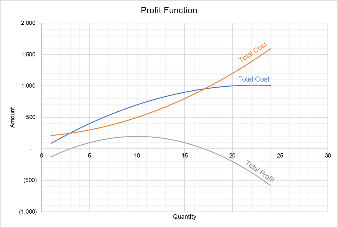
The profit curve plotted above is arrived at by subtracting the total cost curve from the total revenue curve. It starts at a point below the x-axis because the firm is making losses at low output (because even its fixed costs are not recovered). The curve initially slopes upwards, reaches a peak when quantity produced is 10 and then starts to fall. The profit is maximized at output of 10.
Since profit maximization occurs at a point at which the marginal revenue (MR) equals marginal cost (MC), we can verify that it is indeed maximized at Q = 10 by solving the marginal revenue and marginal cost functions (which are obtained by differentiating the total revenue and total cost functions with respect to Q).
$$ \text{MC}\ =\ \text{4Q}\ +\ \text{10}=\text{MR}\ =\ \text{90}\ -\ \text{4Q} $$
$$ \text{4Q}\ +\ \text{4Q}=\text{90}\ - \text{10} $$
$$ \text{Q}=\text{10} $$
by Obaidullah Jan, ACA, CFA and last modified on