Cost Functions
A cost function is a mathematical relationship between cost and output. It tells how costs change in response to changes in output.
Even though relationship between a firm’s costs and output can be studies using cost tables (which show total cost, total variable cost and marginal cost for each unit) or graphs which plot different cost curves, a cost function is the most compact and direct method of encapsulating information about a firm’s costs.
Cost functions typically have cost as a dependent variable and output i.e. quantity as an independent variable. Such cost functions do not account for any changes in cost of inputs because they assume fixed input prices.
Types of Cost Functions
Typical cost functions are either linear, quadratic and cubic.
A linear cost function is such that exponent of quantity is 1. It is appropriate only for cost structures in which marginal cost is constant.
A quadratic cost function, on the other hand, has 2 as exponent of output. It represents a cost structure where average variable cost is U-shaped.
A cubic cost function allows for a U-shaped marginal cost curve. The cost function in the example below is a cubic cost function.
Total cost function is the most fundamental output-cost relationship because functions for other costs such as variable cost, average variable cost and marginal cost, etc. can be derived from the total cost function.
Example
Imagine you work at a firm whose total cost (TC) function is as follows:
$$ \text{TC}\ =\ \text{0.1Q}^\text{3}-\ \text{2Q}^\text{2}+\text{60Q}+\text{200}\ $$
Average total cost function can be derived by dividing the total cost function by Q:
$$ \text{ATC}\ =\ \frac{\text{TC}}{\text{Q}}=\text{0.1Q}^\text{2}-\ \text{2Q}+\text{60}+\frac{\text{200}}{\text{Q}}\ $$
The constant value in a total cost function represent the total fixed cost. Function for total variable cost can be arrived at by subtracting the constant value from the total cost function:
$$ \text{VC}=\text{TC}\ -\ \text{FC}\ $$
$$ \text{VC}=\ \text{0.1Q}^\text{3}-\ \text{2Q}^\text{2}+\text{60Q} $$
Average variable cost function equals total variable cost divided by Q:
$$ \text{AVC}=\frac{\text{VC}}{\text{Q}}=\ \text{0.1Q}^\text{2}-\ \text{2Q}+\text{60} $$
Marginal cost equals the slope of the total cost curve which in turn equals the first derivative of the total cost function.
$$ {\text{MC}} _ \text{Q}=\frac{\text{dTC}}{\text{dQ}}\ =\ \text{0.3Q}^\text{2}-\ \text{4Q}+\text{60}\ $$
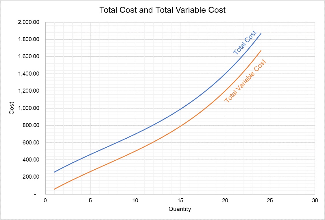
Cost functions can be used to create cost tables and cost curves. By plugging different quantity levels in the cost functions determined above, we can create a cost table which can be used to plot the cost curves.
The total cost and total variable cost curves represented by functions discussed above give us the following graph:
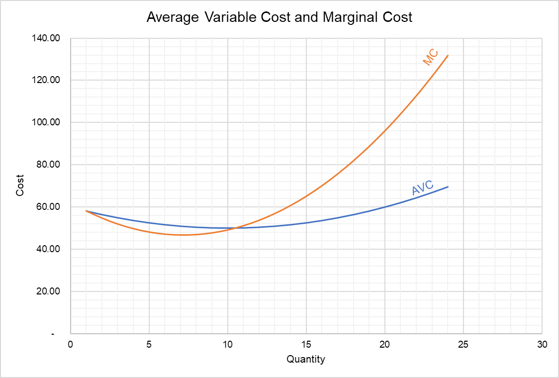
Since the total cost function is a cubic-function, the average variable cost curve and the marginal cost curve are U-shaped as shown below.
by Obaidullah Jan, ACA, CFA and last modified on