Solow Growth Model
Solow growth model is a model that explains the relationship between economic growth and capital accumulation and concludes that economies gravitate towards a steady state of capital and output in the long-run.
Solow growth model is a neoclassical model of growth theory developed by MIT economist Robert Solow. It implies that it is possible for economies to grow in the short run by increasing capital per worker but not in the long run because in the long-run the level of capital is restricted by the income level and savings rate. The model shows that in the long run continuous technological progress is the only engine of growth because it increases total income and eventually the capital and output level.
Example
Let’s consider Dorne whose economy is best explained by the following Cobb-Douglas production function:
$$ \text{Y}=\text{A}\times \text{K}^\frac{\text{1}}{\text{3}}\times \text{L}^\frac{\text{2}}{\text{3}} $$
Y is the total output, A is total factor productivity i.e. a measure of technological progress, K refers to units of capital and L refers to the work force.
Let’s assume (a) Dorne’s only capital good is its irrigation system measured in number of miles of irrigation canals, (b) it’s only produce is cotton and (c) it’s population, labor participation rate and employment rate are constant.
We can write the production function in per-worker terms as follows:
$$ \frac{\text{Y}}{\text{L}}\\=\text{A}\times \text{K}^\frac{\text{1}}{\text{3}}\times \text{L}^\frac{\text{2}}{\text{3}}\div \text{L}\\=\text{A}\times \text{K}^\frac{\text{1}}{\text{3}}\times \text{L}^{\frac{\text{2}}{\text{3}}-\text{1}}\\=\text{A}\times \text{K}^\frac{\text{1}}{\text{3}}\times \text{L}^{-\frac{\text{1}}{\text{3}}}\\=\text{A}\times\left(\frac{\text{K}}{\text{L}}\right)^\frac{\text{1}}{\text{3}} $$
It means that the output per worker depends on the capital per worker i.e. the capital to labor ratio and the share of capital in production. The exponent of 1/3 implies that a one unit increase in capital causes only a fractional increase in output per worker. In other words, as we increase capital per worker, total output per worker increases less and less due to diminishing marginal product of capital.
Let’s imagine the irrigation canals depreciate at a rate of δ each period. It means that the stock of irrigation canals per worker after each period decreases by a factor of δ × K/L. Where k = K/L, this can be expressed as follows:
$$ \delta \text{k}\ =\ \delta\times\ \text{k} $$
To offset the deterioration of their capital, Dornishmen must invest in new canals but their investment capability per worker depends on their income per worker Y/L and savings rate s.
$$ \text{i}\ =\ \text{s}\times\ \text{y} $$
Depreciation rate, capital level, saving rate and output together determine the net change in capital (∆k):
$$ \Delta \text{k}=\text{i} - δ\text{k} = \text{sy} - δ\text{k} $$
Steady State
Output per worker y grows less and less with increase in capital per worker k till it reaches a point when the net change in capital approaches zero. Such a state of zero net change in capital and zero growth in output per worker is called the steady state of capital. It is the level of capital per worker at which the economy has maximized its output per worker.
Let’s illustrate this point using the following data provided by the accountant of House Martell:
- Opening stock of canals is 200 miles and number of workers is 1,000 which remains constant.
- The depreciation rate is 10% i.e. 10% of canals must be reconstructed each period.
- Savings rate is 40%
Using the above information, we can create a table showing the relationship between capital, output, investment and depreciation:
| Period | k | y | i = s × y | δk |
|---|---|---|---|---|
| 1 | 0.20 | 0.58 | 0.23 | 0.02 |
| 2 | 0.41 | 0.75 | 0.30 | 0.04 |
| 3 | 0.67 | 0.88 | 0.35 | 0.07 |
| 4 | 0.95 | 0.98 | 0.39 | 0.10 |
| 5 | 1.25 | 1.08 | 0.43 | 0.13 |
| 75 | 7.93 | 1.99 | 0.80 | 0.79 |
| 76 | 7.94 | 1.99 | 0.80 | 0.79 |
| 77 | 7.94 | 1.99 | 0.80 | 0.79 |
| 78 | 7.94 | 2.00 | 0.80 | 0.79 |
| 79 | 7.95 | 2.00 | 0.80 | 0.79 |
| 80 | 7.95 | 2.00 | 0.80 | 0.80 |
In Period 1, capital per worker of 0.2 generates output of 0.58 (i.e. (0.2)1/3). Since 40% of the output is saved and invested, new investment per worker is 0.23 (i.e. 40% of 0.58) but as 10% of the capital stock depreciates net increase in capital worker is only 0.21 (i.e. 0.23 minis 0.02) and closing stock of capital per worker is 0.41.
In Period 2, capital per worker is 0.41, hence output is 0.75 (=(0.41)1/3), new investment per worker is 0.30 (i.e. 40% of 0.75) but net investment is only 0.26 because 0.04 of capital is depreciated.
This process continues till the economy reaches a point at which new investment and depreciation are equal and there is no increase in capital.
Solow Diagram
If we plot data from the above table, we get a Solow diagram which is a plot with capital per worker on x-axis and output, investment and depreciation on y-axis. It shows the diminishing return to capital and steady state of capital.
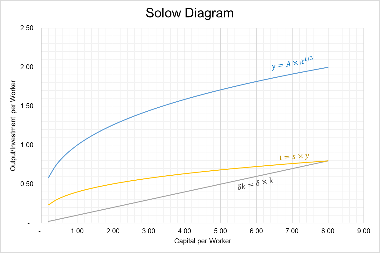
The Solow diagram above shows that as the capital per worker reaches 8, output settles at 2 per worker and remains there infinitely unless there is any change external factor such as war or some natural disaster disturbs the capital per worker. Another factor that changes steady state level of capital is a change in savings rate because it shifts the new investment per worker curve.
The only ingredient that can generate sustained economic growth is technological progress. Technological progress increases total factor productivity which triggers an increase output per worker which in turn increases new investment and the economy moves to a new steady state of capital.
by Obaidullah Jan, ACA, CFA and last modified on