IS-LM Model
IS-LM model is a macroeconomic model that links the output level of an economy in the short-run with interest rate determined by the interplay of fiscal policy and monetary policy in the goods market and financial market.
IS-LM model combines the equilibrium in the goods market with equilibrium in the financial market to reach the mutual equilibrium of both markets. The IS part of the model which stands for ‘investment-saving’ relates to the relationship between demand for goods and interest rate. The LM part of the model which stands for ‘liquidity-money’ represents the relationship between output and interest rate.
IS-LM model applies to short-run because it assumes prices are sticky. It means that the IS-LM model assumes that prices, wages and money supply are given and do not change. The model offers a very useful explanation of the short-run fluctuations because stickiness of prices and wages is indeed the case in the short-run.
IS-LM model was initially developed in 1937 by John Hicks based on works of John Maynard Keynes. An extension of the IS-LM model which integrates the net exports part of aggregate demand with domestic goods market and financial market is called Mundell-Fleming Model or IS-LM-BoP model.
Graph
IS-LM model is graphically represented by a plot of IS and LM curves with interest rate on y-axis and output level on x-axis.
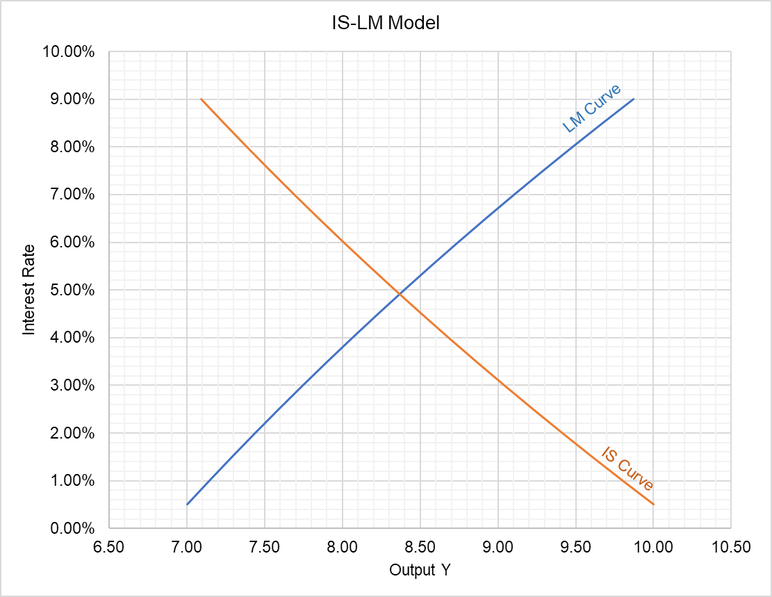
The IS curve slopes downward because an economy’s output is higher at lower interest rate and vice versa.
The LM curve slopes upwards because when output level is higher there is higher demand for money which causes interest rates to be higher.
As shown by the graph above, the interplay of IS curve and LM curve determines the interest rate and output level that prevails in an economy.
Fiscal Policy and Monetary Policy
Changes in fiscal policy such as changes in government spending and changes in taxes shift the IS curve by changing the level of consumption, investment and government spending. If the changes are such that it increases any component of the aggregate expenditure, the IS curve shifts outwards and vice versa.
Monetary policy changes such as purchase or sale of bonds by the central bank or changes in discount rate, etc. also shift the LM curve. If there is a monetary expansion i.e. increase in money supply, the LM curve shifts outwards and it increases output.
The new short-run equilibrium occurs at the point of intersection of the new IS and LM curves.
Example
Let’s consider an economy which undergoes fiscal expansion, an increase in government spending or decrease in taxes, and monetary contraction, a decrease in money supply, at the same time.
A fiscal expansion shifts the IS curve outwards i.e. from IS1 to IS2. The extent on the shift depends on the action causing the shift and any associated multiplier effect.
A monetary contraction, on the other hand, shifts the LM curve inwards, from LM1 to LM2.
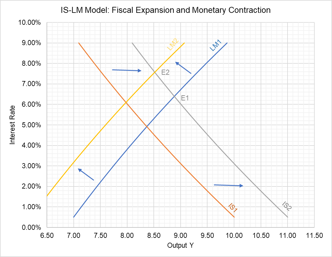
Looking at the graph above, we can see that the equilibrium has moved from E1, the point of intersection of IS1 and LM1 to E2, the point of intersection of IS2 and LM2. The new equilibrium E2 corresponds to a higher interest rate and lower output.
by Obaidullah Jan, ACA, CFA and last modified on