Histogram Equalization
Histogram equalization is an image processing technique which transforms an image in a way that the histogram of the resultant image is equally distributed, which in result enhances the contrast of the image. An equalized histogram means that probabilities of all gray levels are equal. In other words, histogram equalization makes an image use all colors in equal proportion.
Method
New Pixel Value = (L − 1) × Cummulative Probability of Original Pixel Value
Note that the above formula gives us a new gray level for each gray level to be replaced.
Steps
- Traverse the image and calculate the probabilities of the individual gray levels and store it in an array[256] on the respective index number.
- Find the cumulative probabilities of the gray levels and multiply with (L-1). This should result in an array[256] containing the mapping of original gray levels (indices) to be replaced by the new gray levels (values at the indices of the array)
- Traverse the image again and replace the old gray values with the new gray values using the array found in step 2.
Derivation
Let’s assume that images are continuous domain and frequency of the gray levels is a random variable.
Now our goal is to find:
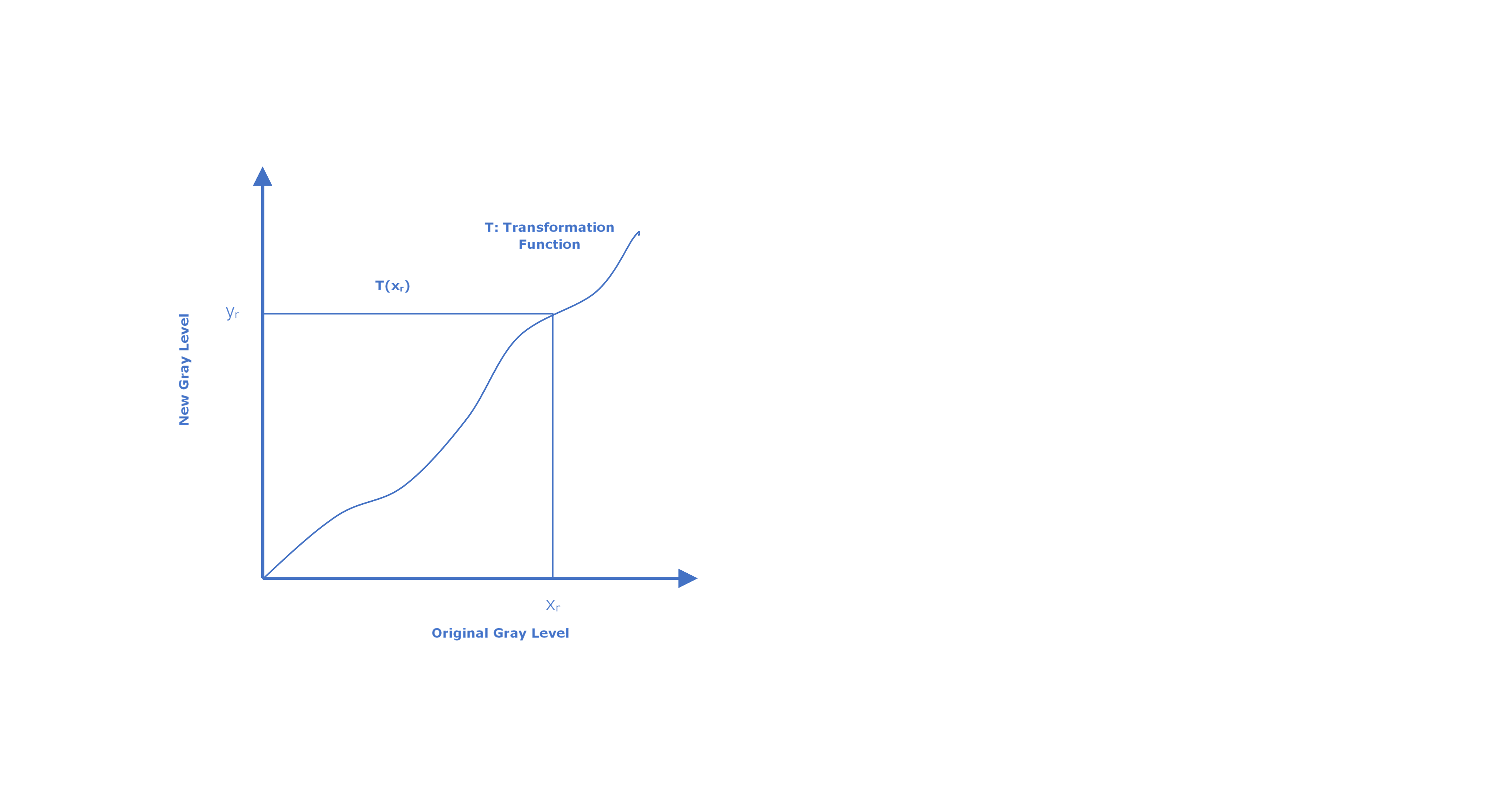
- A mapping function y=f(x) which tells a new value of gray (y) for some value of pixel (x)
- The mapping function should be single valued and monotonically increasing.
- A transformation which maps the gray levels in the same range.
Let px(x), py(y) be the probability density functions for the input image and output image respectively.
As we want the transformation function to map the gray values in the same range:
$$ \text{p} _ \text{y dy}{=\text{p}} _ \text{x dx} $$
The above equation means that the transformation function will result in an image in which the gray levels will be mapped to a wider range (dy) and with a low py(y) if the px(x) is high to maintain the equality and vice versa.
Now py(y) needs to be 1 so that the cumulative probability of the output image is 1.
$$ \int _ {\text{0}}^{\text{1}}{\text{p} _ \text{ydy}}\ =\text{1}=\int _ {\text{0}}^{\text{1}}{(\text{1})\ \text{dy}} $$
Hence
$$ \text{dy}\ =\ \text{p} _ \text{xdx} $$
$$ \int _ {\text{0}}^{\text{y}}\text{dy}\ =\int _ {\text{0}}^{\text{x}}{\text{p} _ \text{x dx}} $$
$$ \text{y}\ =\ \int _ {\text{0}}^{\text{x}}{\text{p} _ \text{x dx}} $$
Hence the new value for a gray level comes from the cumulative probability of that gray level.
Note that the above formula is for continuous domain. It can be represented in discrete domain as follows
$$ \text{y} _ \text{r}\ =\ \sum _ {\text{0}}^{\text{r}}{\text{p} _ \text{x}(\text{x} _ \text{r})} $$
Example
The following image has a bad contrast. Let’s see how histogram equalization of this image helps.
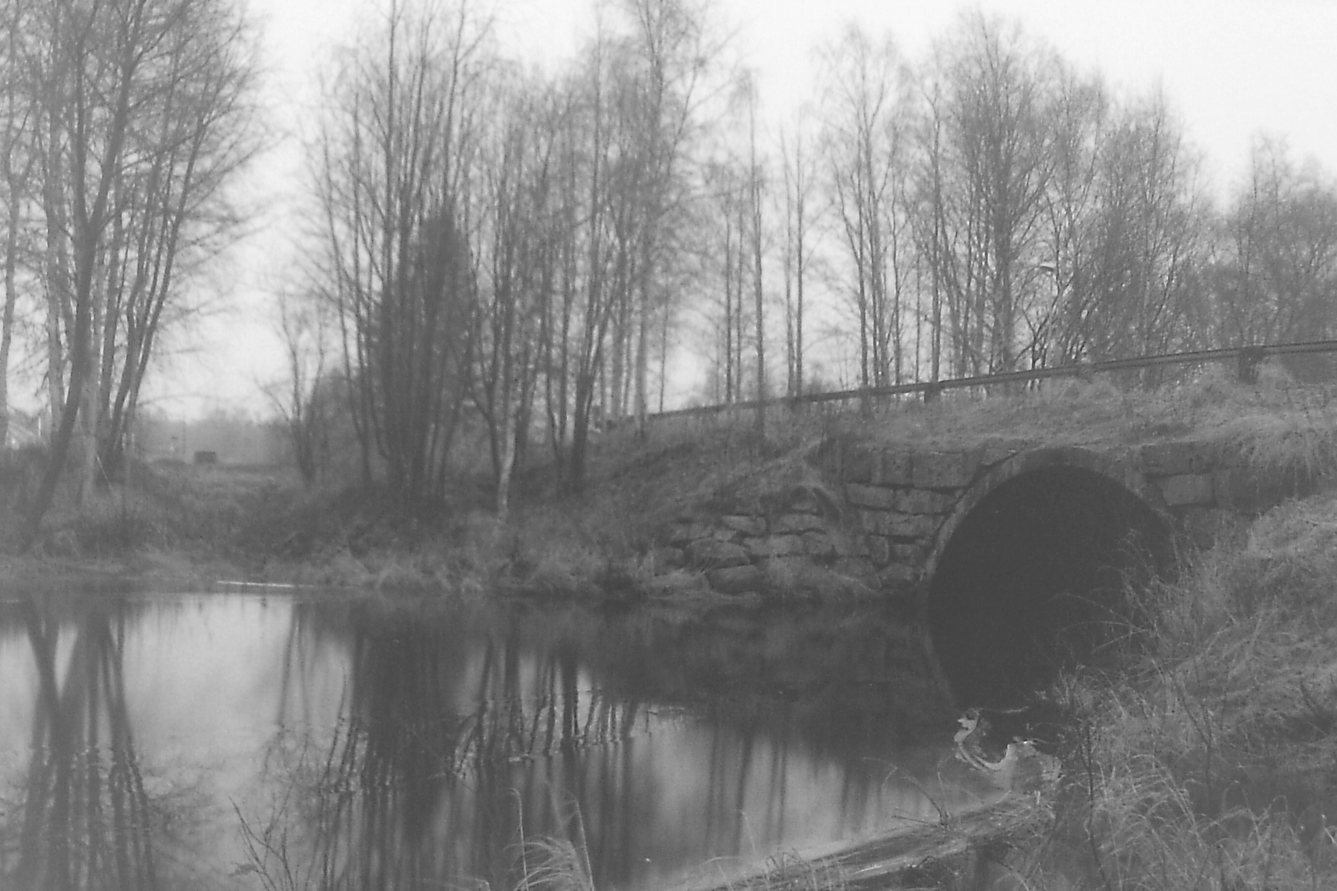

The original histogram is shifted towards white gray levels and is not using any of the gray level till 75. This shows that histogram equalization of the image will give us an image which will equally use all gray levels and will be in high contrast.
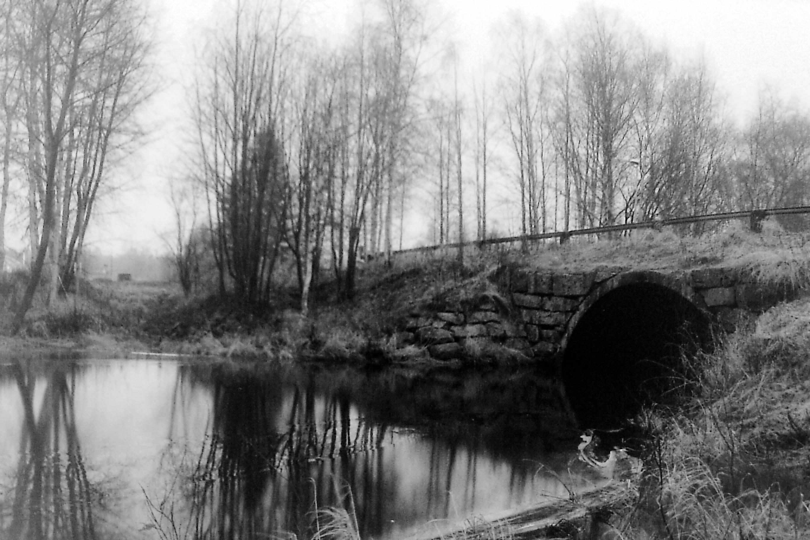

Note: The histogram is not perfectly flat is because of the approximation we did for discrete domain. The formula works perfectly in continuous domain. Although the histogram is not perfectly flat, histogram equalization increases the contrast because the resultant image makes use of all available gray levels.
Code
by Arifullah Jan and last modified on